
Machine Learning Fundamentals in Python
A GradientBoostingClassifier model is fitted on the training data X_train and y_train, and stored as model. Use model and the X_test feature data to predict values for the response variable, and store it in y_pred.
from sklearn.ensemble import GradientBoostingClassifier
from sklearn.metrics import accuracy_score

model = GradientBoostingClassifier(n_estimators=300, max_depth=1, random_state=1)
model.fit(X_train, y_train)

y_pred = model.predict(X_test)
print(accuracy_score(y_test, y_pred))
0.95
0.95
You are supplied with 2 sets of variables; y_pred are predicted using the model supplied and y_test are the actual response values.
Print the main classification metrics for the model.
from sklearn.tree import DecisionTreeClassifier
from sklearn import metrics

model = DecisionTreeClassifier(max_depth=4, random_state=42)

model.fit(X_train, y_train)

y_pred = model.predict(X_test)

print(metrics.classification_report(y_test, y_pred ))
              precision    recall  f1-score   support

           0       0.93      0.94      0.94        54
           1       0.97      0.96      0.96        89

    accuracy                           0.95       143
   macro avg       0.95      0.95      0.95       143
weighted avg       0.95      0.95      0.95       143
3 out of 15
To understand the impact of weekly income on the amount a family spends each week on groceries, fit a suitable model using the weekly_spend data. What is the value of the intercept of the model?
   spend  income  children  car
0     20   19549         0    0
1     52   95248         1    1
2     18   27693         0    1
3     37   50788         1    1
4     46   50312         0    1
import numpy as np
from sklearn.linear_model import LinearRegression

X=np.array(weekly_spend['income']).reshape(-1,1)

mod=LinearRegression()
mod=LinearRegression(fit_intercept=True)

mod.fit(X, y)
mod.fit(X, weekly_spend["spend"])

print(mod.intercept_.round(2))
14.39
Traceback (most recent call last):
  File "<stdin>", line 8, in <module>
    mod.fit(X, y)
NameError: name 'y' is not defined
4 out of 15
A random forest model has been fitted to train data.
Use the results from a random forest classifier to determine the importance of each feature in determining whether a patient does or does not have heart disease.
import matplotlib.pyplot as plt
import seaborn as sns
from sklearn.ensemble import RandomForestClassifier

model = RandomForestClassifier(n_estimators=15,
                               random_state=1)
model.fit(X_train, y_train)

# Create a DataFrame with the feature importances
feature_importances = pd.DataFrame(
    {"feature": list(X.columns), "importance": model.feature_importances_}
).sort_values("importance", ascending=False)

sns.barplot(data=feature_importances, x="importance", y="feature")
plt.show()
5 out of 15
Available in your working session is the dataset scaled_samples. Instantiate a principal component analysis model object with 2 components, and fit the model to the scaled_samples object.
from sklearn.decomposition import PCA

pca = PCA(n_components=2)
pca.fit(scaled_samples)

pca_features = pca.transform(scaled_samples)
print(pca_features.shape)
(85, 2)
6 out of 15
As part of a brainstorming session for a medical startup idea that predicts the chance of diabetes based on a few key readings, you have a sample DataFrame named df with key readings for diabetes:
   Glucose  BloodPressure  Insulin
0      148             72        0
1       85             66        0
2      183             64        0
3       89             66       94
4       78             50      168
Apply Min-Max scaling so that all numeric columns are between 0 and 1.
from sklearn.preprocessing import MinMaxScaler

min_max = MinMaxScaler()
df_scaled = pd.DataFrame(min_max.fit_transform(df), columns=df.columns)
print(df_scaled.head())
   BloodPressure   Glucose   Insulin
0       1.000000  0.666667  0.000000
1       0.727273  0.066667  0.000000
2       0.636364  1.000000  0.000000
3       0.727273  0.104762  0.559524
4       0.000000  0.000000  1.000000
7 out of 15
Create and fit random forest classifier with 15 trees to predict whether a patient has or does not have heart disease. The data has already been split into train and test sets (X_train, X_test, y_train, y_test).
from sklearn.ensemble import RandomForestClassifier
from sklearn.metrics import accuracy_score

model = RandomForestClassifier(n_estimators=15,
                               random_state=1)
model.fit(X_train, y_train)

y_pred = model.predict(X_test)
print(accuracy_score(y_test, y_pred))
0.8032786885245902
8 out of 15
The scatterplot shows data for a sample of 14 biofuels. Fit a linear regression model and print the intercept and coefficient.
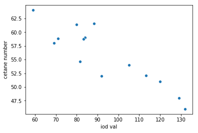
from sklearn.linear_model import LinearRegression

model = LinearRegression(fit_intercept=True)

model.fit(x, y)

print("Regression coefficients: {}".format(model.coef_))
print("Regression intercept: {}".format(model.intercept_))
Regression coefficients: [[-0.20938742]]
Regression intercept: [75.21243193]
9 out of 15
Consider the first five rows of the data frame df shown below. Apply a pre-processing step to standardize all numeric features.
  Sepal.Length Sepal.Width Petal.Length Petal.Width Species
1          5.1         3.5          1.4         0.2  setosa
2          4.9         3.0          1.4         0.2  setosa
3          4.7         3.2          1.3         0.2  setosa
4          4.6         3.1          1.5         0.2  setosa
5          5.0         3.6          1.4         0.2  setosa
6          5.4         3.9          1.7         0.4  setosa
from sklearn.preprocessing import StandardScaler

scaler = StandardScaler()
df_scaled = pd.DataFrame(scaler.fit_transform(df), columns=df.columns)
print(df_scaled.head())
   sepal length (cm)  sepal width (cm)  petal length (cm)  petal width (cm)
0          -0.900681          1.019004          -1.340227         -1.315444
1          -1.143017         -0.131979          -1.340227         -1.315444
2          -1.385353          0.328414          -1.397064         -1.315444
3          -1.506521          0.098217          -1.283389         -1.315444
4          -1.021849          1.249201          -1.340227         -1.315444
10 out of 15
Using the original data, df, training (X_train, y_train) and test (X_test, y_test) sets have been created. Complete the code using the data sets in the appropriate places.
from sklearn.linear_model import LinearRegression
from sklearn.metrics import mean_squared_error

lin_reg = LinearRegression()
lin_reg.fit(X_train,y_train)
predictions = lin_reg.predict(X_test)
print("Mean squared error: %.2f" % mean_squared_error(y_test, predictions))
Mean squared error: 8.47
11 out of 15
A dataset has been prepared for you and split into test and training sets (X_train, X_test, y_train, y_test).
Use sklearn to fit a classification gradient boosting model on the training data with 300 estimators and 0.01 learning rate
from sklearn.ensemble import GradientBoostingClassifier

model = GradientBoostingClassifier(n_estimators=300, learning_rate=0.01, random_state=42)
model.fit(X_train, y_train)

y_pred = model.predict(X_test)

print(model.score(X_test, y_test))
0.8888888888888888
12 out of 15
A dataset has been prepared for you and fed into a random forest model.
Use sklearn to show the predicted probabilities of a new data point belonging to each class.
>>> print(new)
Alcohol    Malic.acid  Phenols Flavanoids
13.64      3.10        2.70    3.01
from sklearn.ensemble import RandomForestClassifier

model = RandomForestClassifier(random_state=42)

model.fit(X_train, y_train)

print(model.predict_proba(new))
[[0. 1. 0.]]
13 out of 15
Consider the data frame df below that shows the total number of observations per month. Fit a suitable imputer to fill the missing values.
Date         Ozone Solar Wind
1976-05-31    26      27      31
1976-06-30    9       30      30
1976-07-31    26      31      31
1976-08-31    26      28      31
1976-09-30    29      30      31
from sklearn.impute import SimpleImputer

imputer = SimpleImputer(strategy='median')

print(imputer.fit(df))
SimpleImputer(add_indicator=False, copy=True, fill_value=None,
              missing_values=nan, strategy='median', verbose=0)
14 out of 15
A linear regression model has been fitted to X_train with respect to y_train.
Test values are provided in the arrays X_test and y_test.
Diagnose potential problems by plotting the residuals against the fitted values, including a lowess smoother.
from matplotlib import pyplot as plt
import seaborn as sns

model = LinearRegression().fit(X_train,y_train)

y_fitted = model.predict(X_test)

sns.residplot(y_test - y_fitted, y_fitted)


plt.show()

15 out of 15
Consider the variable x in the Pandas DataFrame df shown in the plot below. Note that the data contains positive and negative values. Apply a suitable transformation to the data.
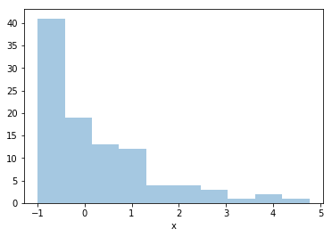
from sklearn.preprocessing import PowerTransformer

log = PowerTransformer(method='yeo-johnson')
df['log_x'] = log.fit_transform(df[['x']])
print(df['log_x'].head())
0   -0.319518
1    1.714791
2    0.823256
3    0.414669
4   -1.054036
Name: log_x, dtype: float64
Retake Assessment
ScoreCompareApr 23rd, 20212:48pmJul 4th, 20213:53pmNoviceIntermediateAdvanced+29 overall134
Your score increased by 29 overall. You started with a score of 105 and just measured 134. Congratulations
Show off your skills and challenge coworkers and friends to do better.LinkedInFacebookTwitter
Your strengths and skill gaps are based on how you performed within each subskill in the assessment.
Strengths
Skill Gaps